library(ISLR)
set.seed(1)
train <- sample(392, 196)Lab 05 Resampling
1 Exploring cross-validation and the bootstrap methods
In this lab, we explore the resampling techniques covered in this chapter. Some of the commands in this lab may take a while to run on your computer.
Validation set concept
We explore the use of the validation set approach in order to estimate the test error rates that result from fitting various linear models on the Auto data set.
Before we begin, we use the set.seed() function in order to set a seed for R’s random number generator, so that the reader of this book will obtain precisely the same results as those shown below. It is generally a good idea to set a random seed when performing an analysis such as cross-validation that contains an element of randomness, so that the results obtained can be reproduced precisely at a later time.
sample()
We begin by using the sample() function to split the set of observations into two halves, by selecting a random subset of 196 observations out of the original 392 observations. We refer to these observations as the training set.
(Here we use a shortcut in the sample command; see ?sample for details.) We then use the subset option in lm() to fit a linear regression using only the observations corresponding to the training set.
lm.fit <- lm(mpg ~ horsepower, data = Auto, subset = train)We now use the predict() function to estimate the response for all 392 observations, and we use the mean() function to calculate the MSE of the 196 observations in the validation set. Note that the -train index below selects only the observations that are not in the training set.
attach(Auto)
mean((mpg - predict(lm.fit, Auto))[-train]^2)
[1] 23.26601Therefore, the estimated test MSE for the linear regression fit is 26.14.
poly()
We can use the poly() function to estimate the test error for polynomial and cubic regressions.
# poly 2nd degree
lm.fit2 <- lm(mpg ~ poly(horsepower, 2),
              data = Auto, subset = train)

mean((mpg - predict(lm.fit2, Auto))[-train ]^2)
[1] 18.71646# poly 3rd degree
lm.fit3 <- lm(mpg ~ poly(horsepower, 3),
data = Auto, subset = train )
mean((mpg - predict(lm.fit3, Auto ))[-train ]^2)[1] 18.79401These error rates are similar to each other, respectively. But, if we choose a different training set instead, then we will obtain somewhat different errors on the validation set.
set.seed(2)
train <- sample(392, 196)

lm.fit <- lm(mpg ~ horsepower, subset = train)
mean((mpg - predict(lm.fit, Auto ))[ -train]^2)
[1] 25.72651lm.fit2 <- lm(mpg ~ poly(horsepower, 2), data = Auto, subset = train)
mean(( mpg - predict( lm.fit2 , Auto ))[ -train]^2)[1] 20.43036lm.fit3 <- lm (mpg ~ poly(horsepower, 3), data = Auto , subset = train)
mean(( mpg - predict (lm.fit3, Auto ))[ -train]^2)[1] 20.38533Although the values are slightly different, these results are consistent with our previous findings: a model that predicts mpg using a quadratic function of horsepower performs better than a model that involves only a linear function of horsepower, and there is little evidence in favor of a model that uses a cubic function of horsepower.
2 Cross validation
Leave-one-out CV
T leave-one-out Cross-validation (LOOCV) estimate can be automatically computed for any generalized linear model using the glm() and cv.glm() functions. We can use the glm() function to perform logistic regression by passing in the family="binomial" argument. But if we use glm() to fit a model without passing in the family argument, then it performs linear regression, just like the lm() function. So for instance,
cv.glm()
# glm() approach
glm.fit <- glm(mpg ~ horsepower, data = Auto)
coef(glm.fit )
(Intercept) horsepower
39.9358610 -0.1578447 # lm() approach
lm.fit <- lm(mpg ~ horsepower, data = Auto)
coef(lm.fit)(Intercept) horsepower
39.9358610 -0.1578447 yield identical linear regression models. In this lab, we will perform linear regression using the glm() function rather than the lm() function because the latter can be used together with cv.glm(). The cv.glm() function is part of the {boot} library.
library(boot)
glm.fit <- glm(mpg ~ horsepower, data = Auto )
cv.err <- cv.glm(Auto, glm.fit)
cv.err$delta
[1] 24.23151 24.23114The cv.glm() function produces a list with several components. The two numbers in the delta vector contain the cross-validation results. In this case the numbers are identical (up to two decimal places) and correspond to the LOOCV statistic (Ch 5 James et al. 2021). Below, we discuss a situation in which the two numbers differ. Our cross-validation estimate for the test error is approximately 24.23.
for()
We can repeat this procedure for increasingly complex polynomial fits. To automate the process, we use the for() function to initiate a for loop which iteratively fits polynomial regressions for polynomials of order i = 1 to i = 5, computes the associated cross-validation error, and stores it in the ith element of the vector cv.error. We begin by initializing the vector. This command will likely take some time to run.
library(tictoc) # time your computer
cv.error <- rep(0 ,5)
tic()
for (i in 1:5){
  glm.fit <- glm(mpg ~ poly(horsepower, i), data = Auto)
  cv.error[i] <- cv.glm(Auto, glm.fit)$delta[1]
}
toc() # Ed's PC
4.78 sec elapsedcv.error[1] 24.23151 19.24821 19.33498 19.42443 19.03321plot(cv.error, type='b')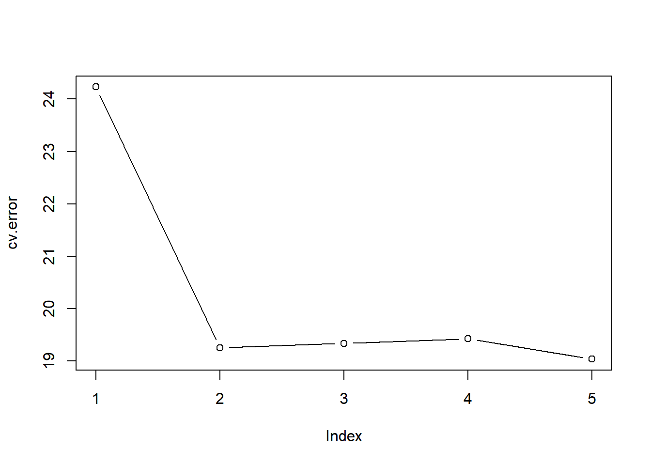
We see a sharp drop in the estimated test MSE between the linear and quadratic fits, but then no clear improvement from using higher-order polynomials.
K-fold CV
The cv.glm() function can also be used to implement k-fold CV. Below we use k = 10, a common choice for k, on the Auto data set. We once again set a random seed and initialize a vector in which we will store the CV errors corresponding to the polynomial fits of orders one to ten.
set.seed(17)
cv.error.10 <- rep (0 ,10)
for(i in  1:10) {
  glm.fit <- glm(mpg ~ poly(horsepower, i), data = Auto )
  cv.error.10[i] = cv.glm(Auto, glm.fit, K = 10)$delta[1]
}
cv.error.10
[1] 24.27207 19.26909 19.34805 19.29496 19.03198 18.89781 19.12061 19.14666
[9] 18.87013 20.95520plot(cv.error.10, type='b')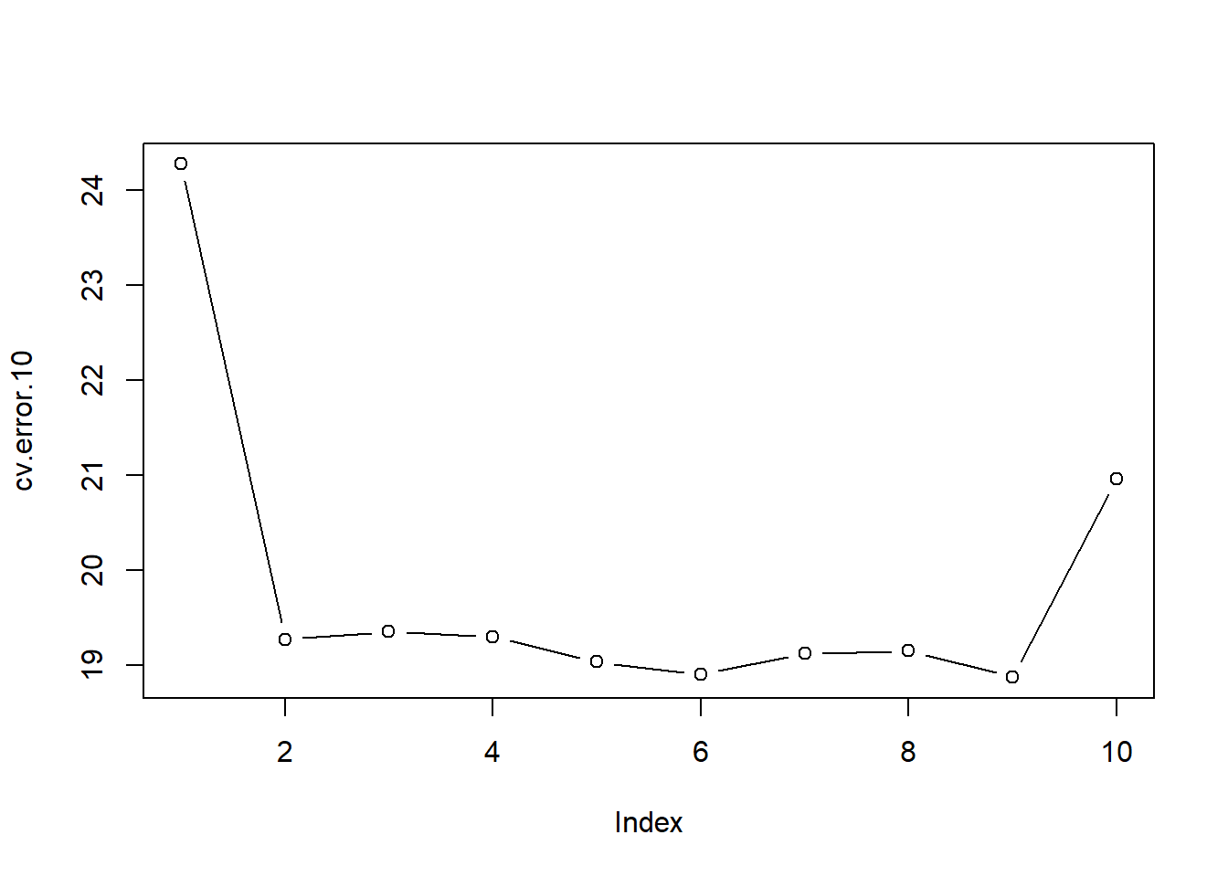
You may notice that the computation time is much shorter than that of LOOCV. (In principle, the computation time for LOOCV for a least squares linear model should be faster than for k-fold CV, due to a mathematical shortcut for LOOCV (see Ch 5 James et al. 2021); however, unfortunately the cv.glm() function does not make use of this efficiency. We still see little evidence that using cubic or higher-order polynomial terms leads to lower test error than simply using a quadratic fit.
The two numbers associated with delta are essentially the same when LOOCV is performed. When we instead perform k-fold CV, then the two numbers associated with delta differ slightly. The first is the standard k-fold CV estimate and the second is a bias-corrected version. On this data set, we see the two estimates are very similar to each other.
3 Bootstrap
We will illustrate the use of the bootstrap in a simple example, as well as on an example involving estimating the accuracy of the linear regression model on the Auto data set.
boot()
One of the great advantages of the bootstrap approach is that it can be applied in almost all situations. No complicated mathematical calculations are required. Performing a bootstrap analysis in R entails only two steps. First, we must create a function that computes the statistic of interest. Second, we use the boot() function, which is part of the {boot} library, to perform the bootstrap by repeatedly sampling observations from the data set with replacement.
The Portfolio data set in the {ISLR} package is described in Section 5.2. To illustrate the use of the bootstrap on this data, we must first create a function, alpha.fn(), which takes as input the (X, Y) data as well as a vector indicating which observations should be used to estimate α. The function then outputs the estimate for α based on the selected observations.
# make a fun function
alpha.fn <- function(data, index){
  X <- data$X[index]
  Y <- data$Y[index]
  return((var(Y) - cov (X, Y))/(var(X)+ var(Y)-2 * cov(X,Y)))
}
This function returns, or outputs, an estimate for α based on the observations indexed by the argument index. For instance, the following command tells R to estimate α using all 100 observations.
alpha.fn(Portfolio, 1:100)[1] 0.5758321The next command uses the sample() function to randomly select 100 observations from the range 1 to 100, with replacement. This is equivalent to constructing a new bootstrap data set and recomputing \(\hat\alpha\) based on the new data set.
set.seed(1)
alpha.fn(Portfolio, sample(100, 100, replace = T))
[1] 0.7368375We can implement a bootstrap analysis by performing this command many times, recording all of the corresponding estimates for α, and computing the resulting standard deviation. However, the boot() function automates this approach. Below we produce R = 1,000 bootstrap estimates for α.
set.seed(1)
boot(Portfolio, alpha.fn, R = 1000)
ORDINARY NONPARAMETRIC BOOTSTRAP


Call:
boot(data = Portfolio, statistic = alpha.fn, R = 1000)


Bootstrap Statistics :
     original       bias    std. error
t1* 0.5758321 -0.001596422  0.09376093
The final output shows that using the original data, \(\hat\alpha= 0.58\), and that the bootstrap estimate for \(SE\hat\alpha = 0.09\).
Regression accuracy
The bootstrap approach can be used to assess the variability of the coef- ficient estimates and predictions from a statistical learning method. Here we use the bootstrap approach in order to assess the variability of the estimates for \(\beta_0\) and \(\beta_1\), the intercept and slope terms for the linear regression model that uses horsepower to predict mpg in the Auto data set. We will compare the estimates obtained using the bootstrap to those obtained using the formulas for \(SE(\hat\beta_0)\) and \(SE(\hat\beta_1)\).
We first create a simple function, boot.fn(), which takes in the Auto data set as well as a set of indices for the observations, and returns the intercept and slope estimates for the linear regression model. We then apply this function to the full set of 392 observations in order to compute the estimates of \(\beta_0\) and \(\beta_1\) on the entire data set using the usual linear regression coefficient estimate formulas. Note that we do not need the { and } at the beginning and end of the function because it is only one line long.
plot(mpg ~ horsepower, data = Auto)
abline(lm(mpg ~ horsepower, data = Auto))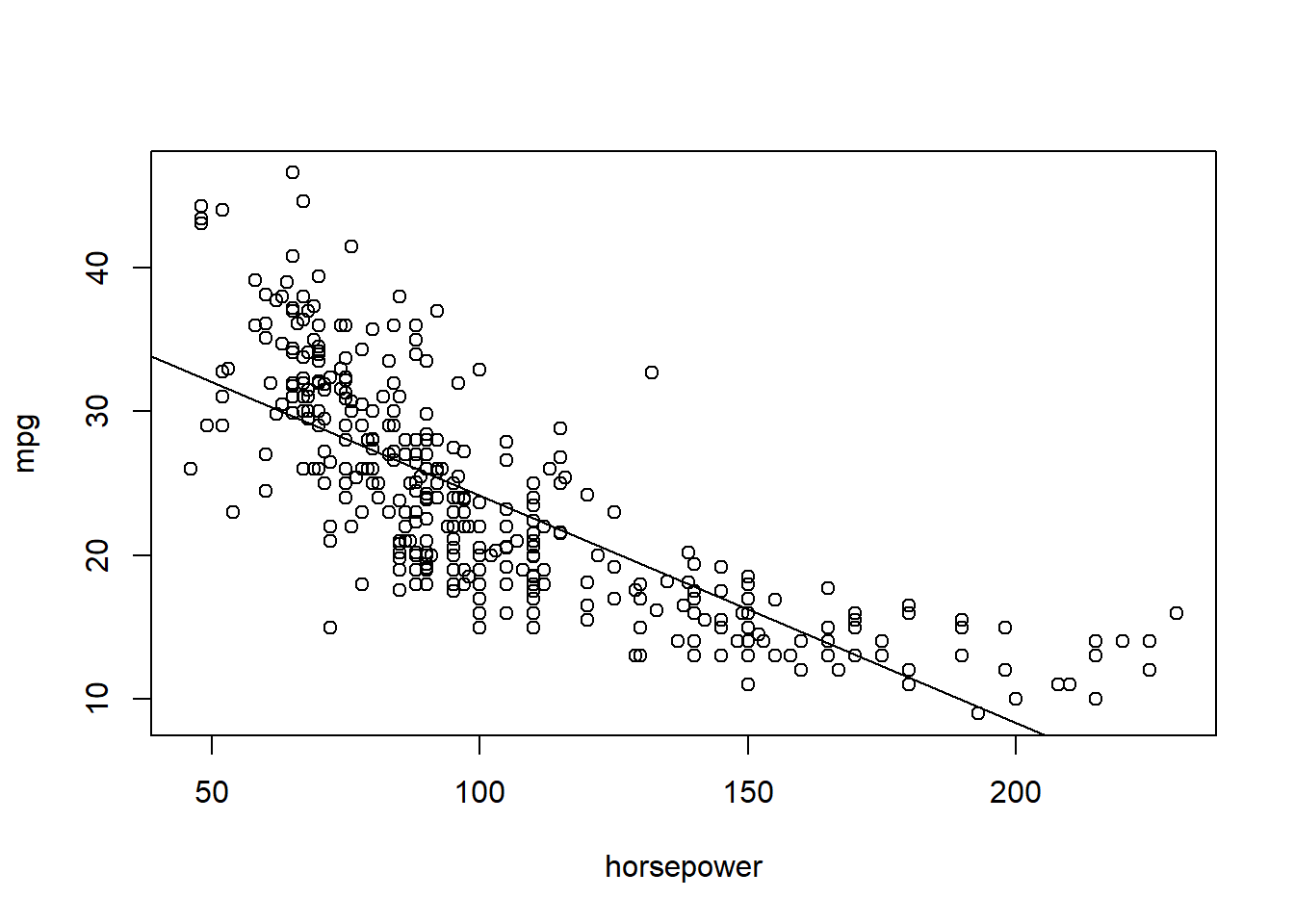
# function!
boot.fn <- function(data, index)
  return(coef(lm(mpg ~ horsepower, data = data, subset = index)))
boot.fn(Auto, 1:392)
(Intercept) horsepower
39.9358610 -0.1578447 The boot.fn() function can also be used in order to create bootstrap estimates for the intercept and slope terms by randomly sampling from among the observations with replacement. Here are two examples:
# first with a seed
set.seed(1)
boot.fn(Auto, sample(392, 392, replace = T))
(Intercept) horsepower
40.3404517 -0.1634868 # no seed
boot.fn(Auto, sample(392, 392, replace = T)) (Intercept) horsepower
40.1186906 -0.1577063 Bootstrap
boot(Auto, boot.fn, 1000)
ORDINARY NONPARAMETRIC BOOTSTRAP


Call:
boot(data = Auto, statistic = boot.fn, R = 1000)


Bootstrap Statistics :
      original        bias    std. error
t1* 39.9358610  0.0544513229 0.841289790
t2* -0.1578447 -0.0006170901 0.007343073
and
This indicates that the bootstrap estimate for \(SE(\hat\beta_0)\) is 0.84, and that the bootstrap estimate for \(SE(\hat\beta_1)\) is 0.0074. Standard formulas can be used to compute the standard errors for the regression coefficients in a linear model. These can be obtained using the summary() function.
summary(lm(mpg ~ horsepower, data = Auto))$coef Estimate Std. Error t value Pr(>|t|)
(Intercept) 39.9358610 0.717498656 55.65984 1.220362e-187
horsepower -0.1578447 0.006445501 -24.48914 7.031989e-81The standard error estimates for \(SE(\hat\beta_0)\) and \(SE(\hat\beta_1)\) somewhat different from the estimates obtained using the bootstrap. Does this indicate a problem with the bootstrap? In fact, it suggests the opposite. Consider that estimation of these parameters rely on certain assumptions. For example, they depend on the unknown parameter \(\sigma^2\), the noise variance. We then estimate \(\sigma^2\) using the RSS. Now although the formula for the standard errors do not rely on the linear model being correct, the estimate for \(\sigma^2\) does. Also, there is a non-linear relationship in the data, and so the residuals from a linear fit will be inflated, and so will \(\sigma^2\). Secondly, standard linear regression assume (somewhat unrealistically) that the \(x_i\) values are fixed, and all the variability comes from the variation in the errors \(\epsilon_i\). The bootstrap approach does not rely on any of these assumptions, and so it is likely giving a more accurate estimate of the standard errors of \(SE(\hat\beta_0)\) and \(SE(\hat\beta_1)\) than is the summary() function.
Below we compute the bootstrap standard error estimates and the standard linear regression estimates that result from fitting the quadratic model to the data. Since this model provides a good fit to the data, there is now a better correspondence between the bootstrap estimates and the standard estimates of \(SE(\hat\beta_0)\), \(SE(\hat\beta_1)\) and \(SE(\hat\beta_2)\).
boot.fn <- function(data, index){
  coefficients(lm(mpg ~ horsepower + I(horsepower^2),
                  data=data,
                  subset = index))
}

set.seed(1)
boot(Auto, boot.fn, 1000)
ORDINARY NONPARAMETRIC BOOTSTRAP


Call:
boot(data = Auto, statistic = boot.fn, R = 1000)


Bootstrap Statistics :
        original        bias     std. error
t1* 56.900099702  3.511640e-02 2.0300222526
t2* -0.466189630 -7.080834e-04 0.0324241984
t3* 0.001230536 2.840324e-06 0.0001172164summary(lm(mpg ~ horsepower + I(horsepower^2), data = Auto))$coef Estimate Std. Error t value Pr(>|t|)
(Intercept) 56.900099702 1.8004268063 31.60367 1.740911e-109
horsepower -0.466189630 0.0311246171 -14.97816 2.289429e-40
I(horsepower^2) 0.001230536 0.0001220759 10.08009 2.196340e-214 Exercises
Exercise 1
We have used logistic regression to predict the probability of default using income and balance on the Default data set. We will now estimate the test error of this logistic regression model using the validation set approach. Do not forget to set a random seed before beginning your analysis.
1.1
Fit a logistic regression model that uses income and balance to predict default.
1.2
Using the validation set approach, estimate the test error of this model. In order to do this, you must perform the following steps:
Split the sample set into a training set and a validation set.
Fit a multiple logistic regression model using only the training observations.
Obtain a prediction of default status for each individual in the validation set by computing the posterior probability of default for that individual, and classifying the individual to the default category if the posterior probability is greater than 0.5.
Compute the validation set error, which is the fraction of the observations in the validation set that are misclassified.
1.3
Repeat the process in 1.2 three times, using three different splits of the observations into a training set and a validation set. Comment on the results obtained.
1.4
Now consider a logistic regression model that predicts the probability of default using income, balance, and a dummy variable for student. Estimate the test error for this model using the validation set approach. Comment on whether or not including a dummy variable for student leads to a reduction in the test error rate.
Resources
Harper Adams Data Science

This module is a part of the MSc in Data Science for Global Agriculture, Food, and Environment at Harper Adams University, led by Ed Harris.