library(MASS)
library(ISLR)Lab 03 Linear regression
1 Setup
library()
The library() function is used to load libraries, or groups of functions and data sets that are not included in the base R distribution. Basic functions that perform least squares linear regression and other simple analyses come standard with the base distribution, but more exotic functions require additional libraries. Here we load the {MASS} package, which is a very large collection of data sets and functions. We also load the {ISLR} package, which includes the data sets associated with James et al. 2001.
If you receive an error message when loading these libraries, it likely indicates that the corresponding library has not yet been installed on your system. Some libraries, such as {MASS}, come with R and do not need to be separately installed on your computer. However, other packages, such as {ISLR}, must be downloaded the first time they are used. This can be done directly from within R. For example, on a Windows system, select the Install package option under the Packages tab. After you select any mirror site, a list of available packages will appear. Simply select the package you wish to install and R will automatically download the package. Alternatively, this can be done at the R command line via install.packages("ISLR"). This installation only needs to be done the first time you use a package. However, the library() function must be called each time you wish to use a given package.
Simple linear regression
The {MASS} library contains the Boston data set, which records medv (median house value) for 506 neighborhoods around the US city of Boston. We will seek to predict medv using 13 predictors such as rm (average number of rooms per house), age (average age of houses), and lstat (percent of households with low socioeconomic status).
names(Boston) [1] "crim" "zn" "indus" "chas" "nox" "rm" "age"
[8] "dis" "rad" "tax" "ptratio" "black" "lstat" "medv" head(Boston) crim zn indus chas nox rm age dis rad tax ptratio black lstat
1 0.00632 18 2.31 0 0.538 6.575 65.2 4.0900 1 296 15.3 396.90 4.98
2 0.02731 0 7.07 0 0.469 6.421 78.9 4.9671 2 242 17.8 396.90 9.14
3 0.02729 0 7.07 0 0.469 7.185 61.1 4.9671 2 242 17.8 392.83 4.03
4 0.03237 0 2.18 0 0.458 6.998 45.8 6.0622 3 222 18.7 394.63 2.94
5 0.06905 0 2.18 0 0.458 7.147 54.2 6.0622 3 222 18.7 396.90 5.33
6 0.02985 0 2.18 0 0.458 6.430 58.7 6.0622 3 222 18.7 394.12 5.21
medv
1 24.0
2 21.6
3 34.7
4 33.4
5 36.2
6 28.7lm()
To find out more about the data set, we can type ?Boston. We will start by using the lm() function to fit a simple linear regression model, with medv as the response and lstat as the predictor. The basic syntax is lm(y∼x,data), where y is the response, x is the predictor, and data is the data set in which these two variables are kept.
# try this
# lm.fit <- lm(medv~lstat)
The command causes an error because R does not know where to find the variables medv and lstat. The next line tells R that the variables are in Boston. If we attach Boston, the first line would work fine because R now recognizes the variables. However, the data argument works here too.
lm.fit <- lm(medv~lstat , data = Boston)
attach(Boston)
lm.fit <- lm(medv~lstat)
If we submit lm.fit, some basic information about the model is output. For more detailed information, we use summary(lm.fit). This gives us p-values and standard errors for the coeffcients, as well as the R2 statistic and F-statistic for the model.
lm.fit
Call:
lm(formula = medv ~ lstat)

Coefficients:
(Intercept)        lstat
34.55 -0.95 summary(lm.fit)
Call:
lm(formula = medv ~ lstat)

Residuals:
    Min      1Q  Median      3Q     Max
-15.168  -3.990  -1.318   2.034  24.500

Coefficients:
            Estimate Std. Error t value Pr(>|t|)
(Intercept) 34.55384    0.56263   61.41   <2e-16 ***
lstat       -0.95005    0.03873  -24.53   <2e-16 ***
---
Signif. codes:  0 '***' 0.001 '**' 0.01 '*' 0.05 '.' 0.1 ' ' 1

Residual standard error: 6.216 on 504 degrees of freedom
Multiple R-squared:  0.5441,    Adjusted R-squared:  0.5432
F-statistic: 601.6 on 1 and 504 DF, p-value: < 2.2e-16names(lm.fit) [1] "coefficients" "residuals" "effects" "rank"
[5] "fitted.values" "assign" "qr" "df.residual"
[9] "xlevels" "call" "terms" "model" coef(lm.fit)(Intercept) lstat
34.5538409 -0.9500494 The predict() function can be used to produce confidence intervals and prediction intervals for the prediction of medv for a given value of lstat.
predict(lm.fit, data.frame(lstat = ( c(5, 10, 15) )),
        interval = "confidence")
fit lwr upr
1 29.80359 29.00741 30.59978
2 25.05335 24.47413 25.63256
3 20.30310 19.73159 20.87461predict(lm.fit, data.frame(lstat = ( c(5, 10, 15) )),
interval = "prediction") fit lwr upr
1 29.80359 17.565675 42.04151
2 25.05335 12.827626 37.27907
3 20.30310 8.077742 32.52846For instance, the 95% confidence interval associated with a lstat value of 10 is (24.47, 25.63), and the 95% prediction interval is (12.828, 37.28). As expected, the confidence and prediction intervals are centered around the same point (a predicted value of 25.05 for medv when lstat equals 10), but the latter are substantially wider.
We will now plot medv and lstat along with the least squares regression line using the plot() and abline() functions.
plot(lstat , medv)
abline(lm.fit)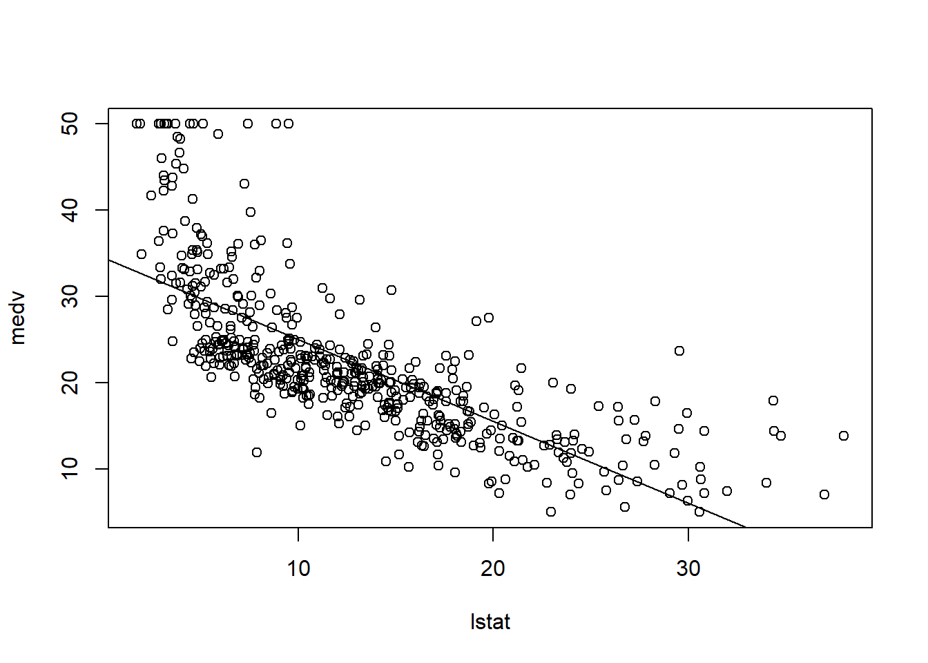
There is some visual evidence for non-linearity in the relationship between lstat and medv. We will explore this issue later in this lab.
The abline() function can be used to draw any line, not just the least squares regression line. To draw a line with intercept a and slope b, we type abline(a,b). Below we experiment with some additional settings for plotting lines and points. The lwd=3 command causes the width of the regression line to be increased by a factor of 3; this works for the plot() and lines() functions also. We can also use the pch option to create different plotting symbols.
plot(lstat , medv)
abline(lm.fit, lwd = 3)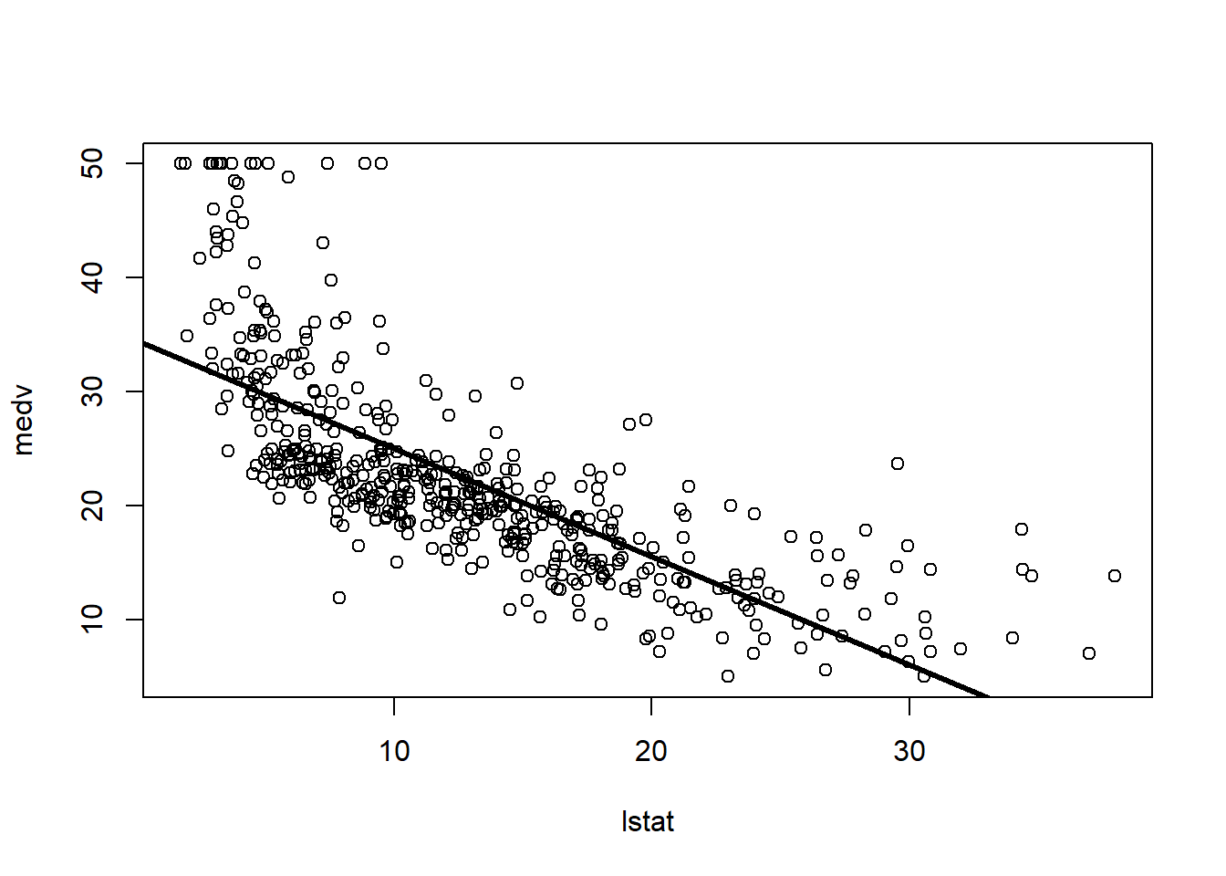
plot(lstat , medv)
abline(lm.fit, lwd = 3, col = "red")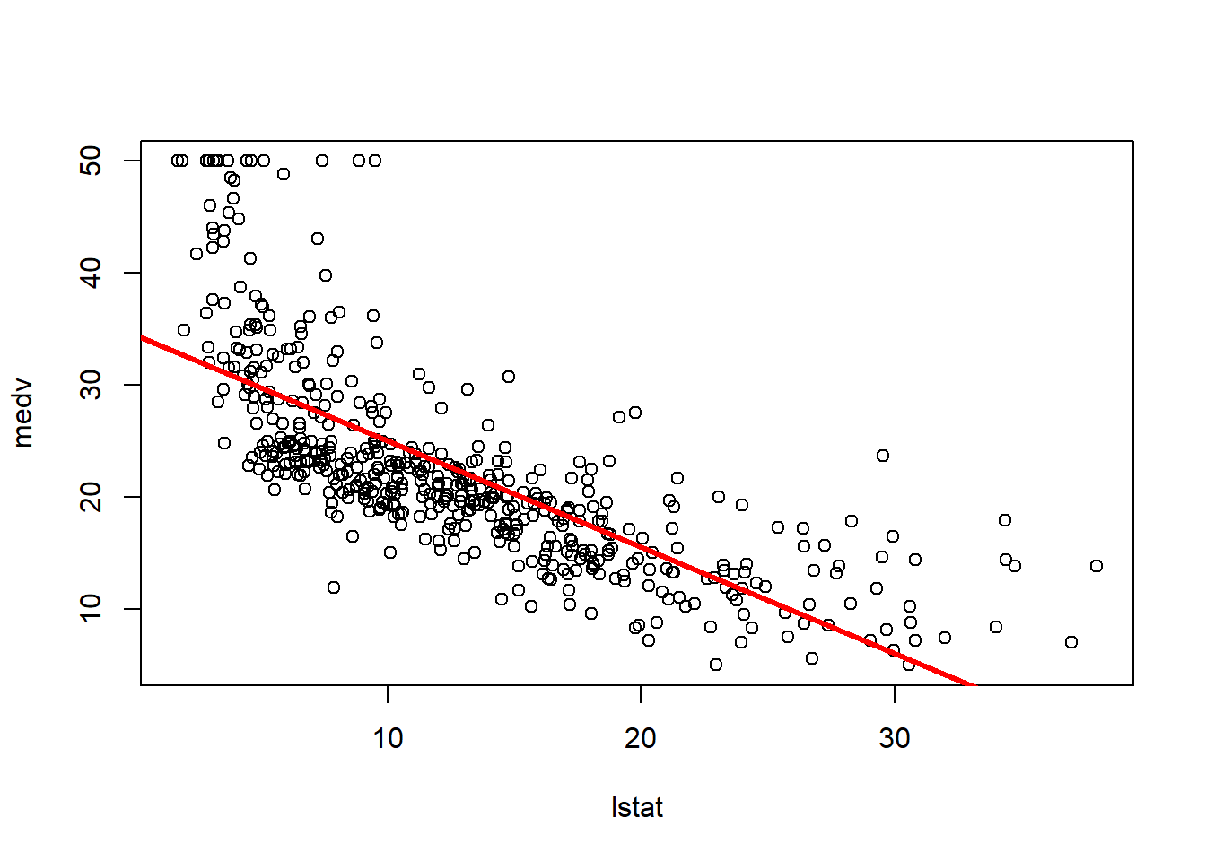
plot(lstat, medv, col = "red")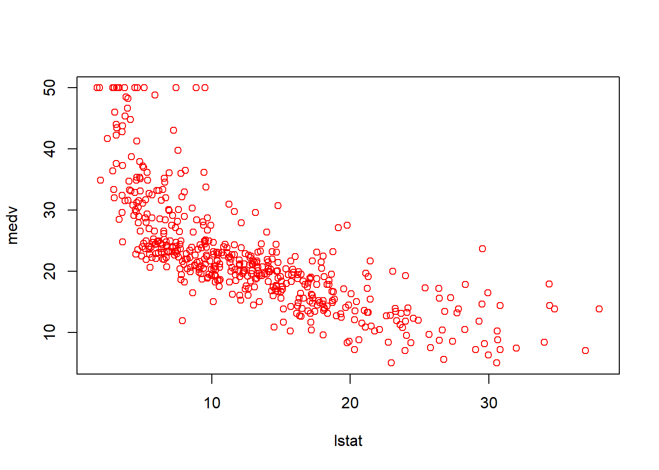
plot(lstat, medv, pch = 20)
plot(lstat, medv, pch ="+")
plot(1:20, 1:20, pch = 1:20)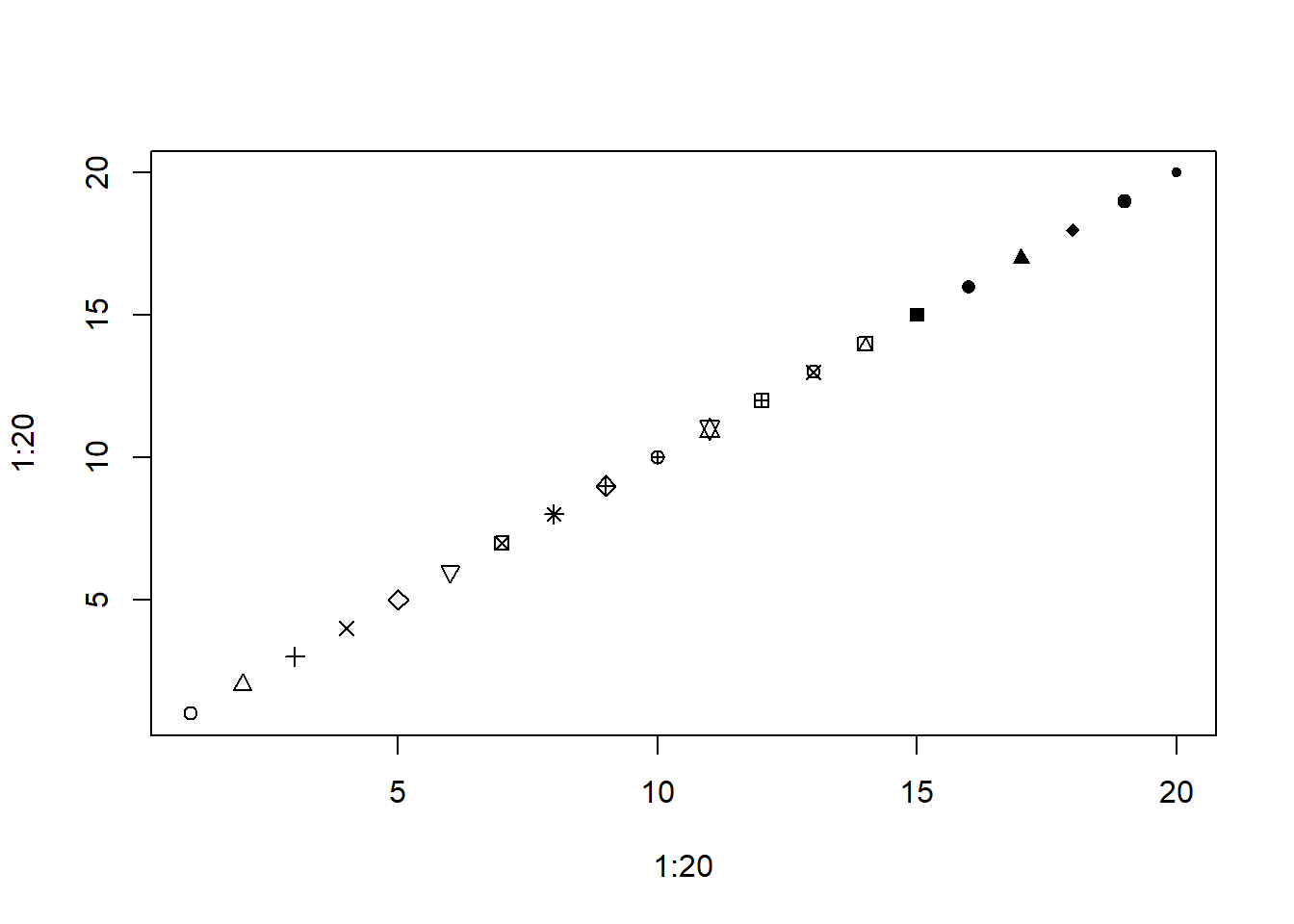
Diagnostic plots
Next we examine some diagnostic plots (discussed in Section 3.3.3 of James et al. 2021). Four diagnostic plots are automatically produced by applying the plot() function directly to the output from lm(). In general, this command will produce one plot at a time, and hitting Enter will generate the next plot. However, it is often convenient to view all four plots together. We can achieve this by using the par() function, which tells R to split the display screen into separate panels so that multiple plots can be viewed simultaneously. For example, par(mfrow=c(2,2)) divides the plotting region into a 2 × 2 grid of panels.
par(mfrow = c(2, 2))
plot(lm.fit)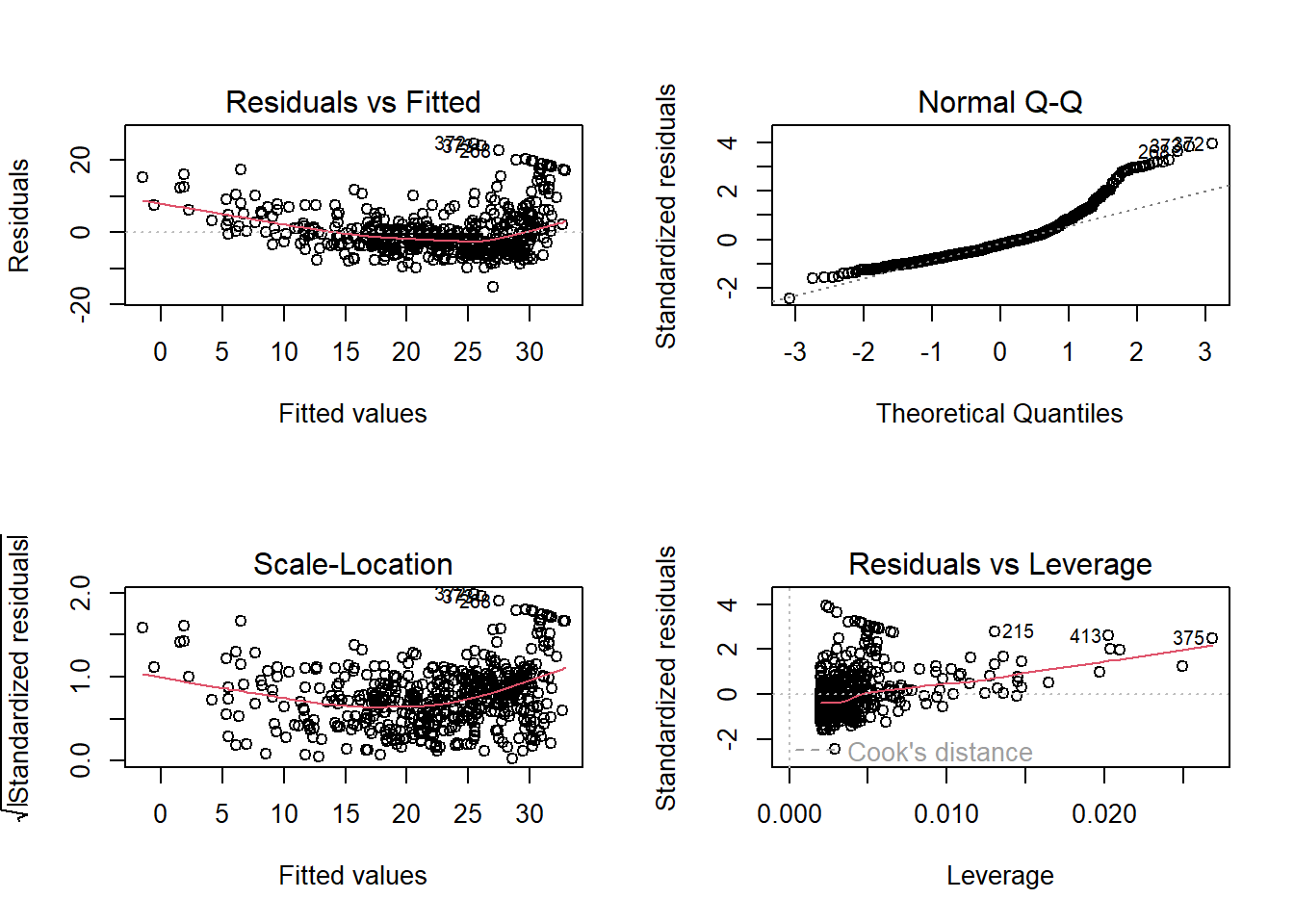
Alternatively, we can compute the residuals from a linear regression fit using the residuals() function. The function rstudent() will return the studentized residuals, and we can use this function to plot the residuals against the fitted values.
par(mfrow = c(1, 3))
plot(predict(lm.fit), residuals(lm.fit))
plot(predict(lm.fit), rstudent(lm.fit))
plot(residuals(lm.fit), rstudent(lm.fit)) # hmm actually these are the same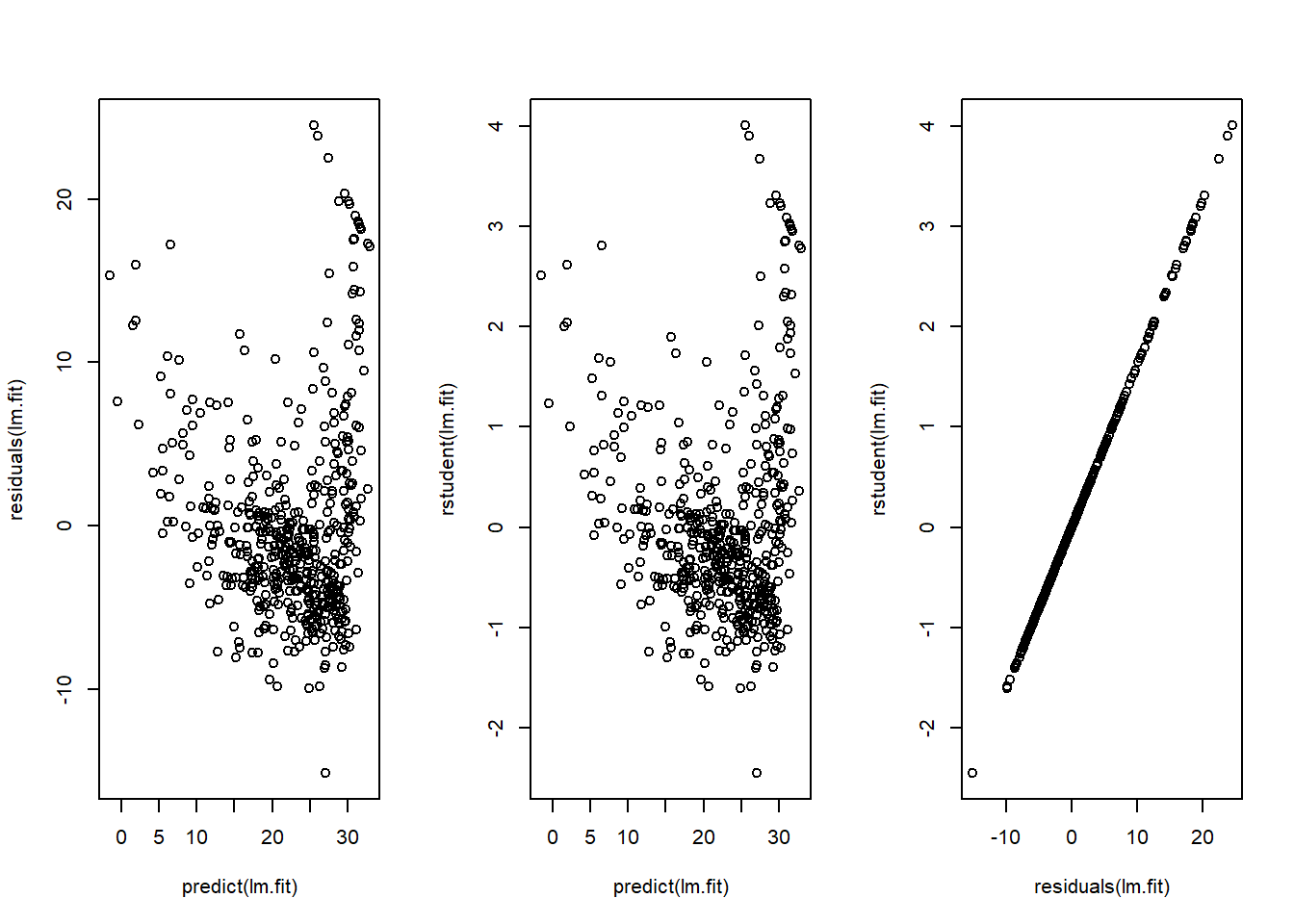
On the basis of the residual plots, there is some evidence of non-linearity. Leverage statistics can be computed for any number of predictors using the hatvalues() function.
par(mfrow = c(1, 1))
plot(hatvalues(lm.fit))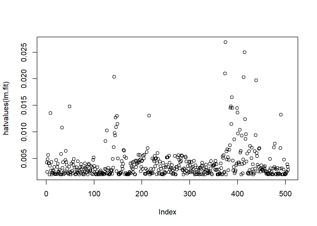
which.max(hatvalues(lm.fit)) 375
375 The which.max() function identifies the index of the largest element of a vector. In this case, it tells us which observation has the largest leverage statistic.
2 Multiple regression
In order to fit a multiple linear regression model using least squares, we again use the lm() function. The syntax lm(y∼x1+x2+x3) is used to fit a model with three predictors, x1, x2, and x3. The summary() function now outputs the regression coefficients for all the predictors.
lm.fit <- lm(medv ~ lstat + age, data = Boston )
summary(lm.fit)
Call:
lm(formula = medv ~ lstat + age, data = Boston)

Residuals:
    Min      1Q  Median      3Q     Max
-15.981  -3.978  -1.283   1.968  23.158

Coefficients:
            Estimate Std. Error t value Pr(>|t|)
(Intercept) 33.22276    0.73085  45.458  < 2e-16 ***
lstat       -1.03207    0.04819 -21.416  < 2e-16 ***
age          0.03454    0.01223   2.826  0.00491 **
---
Signif. codes:  0 '***' 0.001 '**' 0.01 '*' 0.05 '.' 0.1 ' ' 1

Residual standard error: 6.173 on 503 degrees of freedom
Multiple R-squared:  0.5513,    Adjusted R-squared:  0.5495
F-statistic:   309 on 2 and 503 DF,  p-value: < 2.2e-16
The Boston data set contains 13 variables, and so it would be cumbersome to have to type all of these in order to perform a regression using all of the predictors. Instead, we can use the following short-hand:
lm.fit <- lm(medv ~ ., data = Boston)
summary(lm.fit)
Call:
lm(formula = medv ~ ., data = Boston)

Residuals:
    Min      1Q  Median      3Q     Max
-15.595  -2.730  -0.518   1.777  26.199

Coefficients:
              Estimate Std. Error t value Pr(>|t|)
(Intercept)  3.646e+01  5.103e+00   7.144 3.28e-12 ***
crim        -1.080e-01  3.286e-02  -3.287 0.001087 **
zn           4.642e-02  1.373e-02   3.382 0.000778 ***
indus        2.056e-02  6.150e-02   0.334 0.738288
chas         2.687e+00  8.616e-01   3.118 0.001925 **
nox         -1.777e+01  3.820e+00  -4.651 4.25e-06 ***
rm           3.810e+00  4.179e-01   9.116  < 2e-16 ***
age          6.922e-04  1.321e-02   0.052 0.958229
dis         -1.476e+00  1.995e-01  -7.398 6.01e-13 ***
rad          3.060e-01  6.635e-02   4.613 5.07e-06 ***
tax         -1.233e-02  3.760e-03  -3.280 0.001112 **
ptratio     -9.527e-01  1.308e-01  -7.283 1.31e-12 ***
black        9.312e-03  2.686e-03   3.467 0.000573 ***
lstat       -5.248e-01  5.072e-02 -10.347  < 2e-16 ***
---
Signif. codes:  0 '***' 0.001 '**' 0.01 '*' 0.05 '.' 0.1 ' ' 1

Residual standard error: 4.745 on 492 degrees of freedom
Multiple R-squared:  0.7406,    Adjusted R-squared:  0.7338
F-statistic: 108.1 on 13 and 492 DF,  p-value: < 2.2e-16
We can access the individual components of a summary object by name (type ?summary.lm to see what is available). Hence summary(lm.fit)$r.sq gives us the R2, and summary(lm.fit)$sigma gives us the RSE. The vif() function, part of the {car} package, can be used to compute variance inflation factors. Most VIF’s are low to moderate for this data (<= 4.0 is considered low). The {car} package is not part of the base R installation so it must be downloaded the first time you use it via the install.packages option in R.
library(car)Loading required package: carDatavif(lm.fit) crim zn indus chas nox rm age dis
1.792192 2.298758 3.991596 1.073995 4.393720 1.933744 3.100826 3.955945
rad tax ptratio black lstat
7.484496 9.008554 1.799084 1.348521 2.941491 What if we would like to perform a regression using all of the variables but one? For example, in the above regression output, age has a high p-value. So we may wish to run a regression excluding this predictor. The following syntax results in a regression using all predictors except age.
lm.fit1 <- lm(medv ~ . -age, data = Boston )
summary(lm.fit1 )
Call:
lm(formula = medv ~ . - age, data = Boston)

Residuals:
     Min       1Q   Median       3Q      Max
-15.6054  -2.7313  -0.5188   1.7601  26.2243

Coefficients:
              Estimate Std. Error t value Pr(>|t|)
(Intercept)  36.436927   5.080119   7.172 2.72e-12 ***
crim         -0.108006   0.032832  -3.290 0.001075 **
zn            0.046334   0.013613   3.404 0.000719 ***
indus         0.020562   0.061433   0.335 0.737989
chas          2.689026   0.859598   3.128 0.001863 **
nox         -17.713540   3.679308  -4.814 1.97e-06 ***
rm            3.814394   0.408480   9.338  < 2e-16 ***
dis          -1.478612   0.190611  -7.757 5.03e-14 ***
rad           0.305786   0.066089   4.627 4.75e-06 ***
tax          -0.012329   0.003755  -3.283 0.001099 **
ptratio      -0.952211   0.130294  -7.308 1.10e-12 ***
black         0.009321   0.002678   3.481 0.000544 ***
lstat        -0.523852   0.047625 -10.999  < 2e-16 ***
---
Signif. codes:  0 '***' 0.001 '**' 0.01 '*' 0.05 '.' 0.1 ' ' 1

Residual standard error: 4.74 on 493 degrees of freedom
Multiple R-squared:  0.7406,    Adjusted R-squared:  0.7343
F-statistic: 117.3 on 12 and 493 DF,  p-value: < 2.2e-16
Alternatively, the update() function can be used.
lm.fit1 <- update(lm.fit , ~ . -age )Interaction terms
it is easy to include interaction terms in a linear model using the lm() function. The syntax lstat:black tells R to include an interaction term between lstat and black. The syntax lstat*age simultaneously includes lstat, age, and the interaction term lstat:age as predictors; it is a shorthand for lstat + age + lstat:age.
summary(lm(medv ~ lstat * age , data = Boston ))
Call:
lm(formula = medv ~ lstat * age, data = Boston)

Residuals:
    Min      1Q  Median      3Q     Max
-15.806  -4.045  -1.333   2.085  27.552

Coefficients:
              Estimate Std. Error t value Pr(>|t|)
(Intercept) 36.0885359  1.4698355  24.553  < 2e-16 ***
lstat       -1.3921168  0.1674555  -8.313 8.78e-16 ***
age         -0.0007209  0.0198792  -0.036   0.9711
lstat:age    0.0041560  0.0018518   2.244   0.0252 *
---
Signif. codes:  0 '***' 0.001 '**' 0.01 '*' 0.05 '.' 0.1 ' ' 1

Residual standard error: 6.149 on 502 degrees of freedom
Multiple R-squared:  0.5557,    Adjusted R-squared:  0.5531
F-statistic: 209.3 on 3 and 502 DF,  p-value: < 2.2e-16
Non-linear transformation of predictors
The lm() function can also accommodate non-linear transformations of the predictors. For instance, given a predictor \(X\), we can create a predictor \(X^2\) using I(X^2). The function I() is needed since the ^ has a special meaning in a formula; wrapping as we do allows the standard usage in R, which is to raise X to the power 2. We now perform a regression of medv onto lstat and lstat\(^2\).
lm.fit2 <- lm( medv ~ lstat + I(lstat^2))
summary(lm.fit2 )
Call:
lm(formula = medv ~ lstat + I(lstat^2))

Residuals:
     Min       1Q   Median       3Q      Max
-15.2834  -3.8313  -0.5295   2.3095  25.4148

Coefficients:
             Estimate Std. Error t value Pr(>|t|)
(Intercept) 42.862007   0.872084   49.15   <2e-16 ***
lstat       -2.332821   0.123803  -18.84   <2e-16 ***
I(lstat^2)   0.043547   0.003745   11.63   <2e-16 ***
---
Signif. codes:  0 '***' 0.001 '**' 0.01 '*' 0.05 '.' 0.1 ' ' 1

Residual standard error: 5.524 on 503 degrees of freedom
Multiple R-squared:  0.6407,    Adjusted R-squared:  0.6393
F-statistic: 448.5 on 2 and 503 DF,  p-value: < 2.2e-16
anova()
The near-zero p-value associated with the quadratic term suggests that it leads to an improved model. We use the anova() function to compare our models to further quantify the extent to which the quadratic fit is superior to the linear fit.
lm.fit <- lm( medv ~ lstat)
anova(lm.fit, lm.fit2)
Analysis of Variance Table
Model 1: medv ~ lstat
Model 2: medv ~ lstat + I(lstat^2)
Res.Df RSS Df Sum of Sq F Pr(>F)
1 504 19472
2 503 15347 1 4125.1 135.2 < 2.2e-16 ***
---
Signif. codes: 0 '***' 0.001 '**' 0.01 '*' 0.05 '.' 0.1 ' ' 1Here Model 1 represents the linear submodel containing only one predictor, lstat, while Model 2 corresponds to the larger quadratic model that has two predictors, lstat and lstat2. The anova() function performs a hypothesis test comparing the two models. The null hypothesis is that the two models fit the data equally well, and the alternative hypothesis is that the full model is superior. Here the F-statistic is 135 and the associated p-value is virtually zero. This provides very clear evidence that the model containing the predictors lstat and lstat\(^2\) is far superior to the model that only contains the predictor lstat (based on the results that the RSS, the unexplained error, is higher in Model 1). This is not surprising, since earlier we saw evidence for non-linearity in the relationship between medv and lstat. If we type
par(mfrow = c(2, 2))
plot(lm.fit2)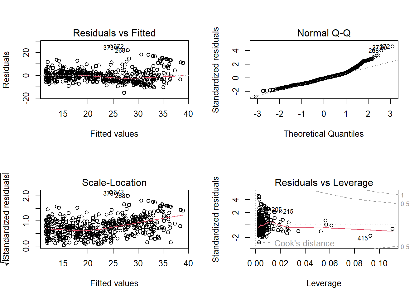
par(mfrow = c(1, 1))then we see that when the lstat\(^2\) term is included in the model, there is little discernible pattern in the residuals.
poly()
In order to create a cubic fit, we can include a predictor of the form I(X^3). However, this approach can start to get cumbersome for higher-order polynomials. A better approach involves using the poly() function to create the polynomial within lm(). For example, the following command produces a fifth-order polynomial fit:
lm.fit5 <- lm(medv ~ poly(lstat, 5))
summary(lm.fit5)
Call:
lm(formula = medv ~ poly(lstat, 5))

Residuals:
     Min       1Q   Median       3Q      Max
-13.5433  -3.1039  -0.7052   2.0844  27.1153

Coefficients:
                 Estimate Std. Error t value Pr(>|t|)
(Intercept)       22.5328     0.2318  97.197  < 2e-16 ***
poly(lstat, 5)1 -152.4595     5.2148 -29.236  < 2e-16 ***
poly(lstat, 5)2   64.2272     5.2148  12.316  < 2e-16 ***
poly(lstat, 5)3  -27.0511     5.2148  -5.187 3.10e-07 ***
poly(lstat, 5)4   25.4517     5.2148   4.881 1.42e-06 ***
poly(lstat, 5)5  -19.2524     5.2148  -3.692 0.000247 ***
---
Signif. codes:  0 '***' 0.001 '**' 0.01 '*' 0.05 '.' 0.1 ' ' 1

Residual standard error: 5.215 on 500 degrees of freedom
Multiple R-squared:  0.6817,    Adjusted R-squared:  0.6785
F-statistic: 214.2 on 5 and 500 DF,  p-value: < 2.2e-16
This suggests that including additional polynomial terms, up to fifth order, leads to an improvement in the model fit! However, further investigation of the data reveals that no polynomial terms beyond fifth order have signifi- cant p-values in a regression fit.
log() transformation
Of course, we are in no way restricted to using polynomial transformations of the predictors. Here we try a log() transformation.
summary(lm(medv~log(rm), data = Boston))
Call:
lm(formula = medv ~ log(rm), data = Boston)

Residuals:
    Min      1Q  Median      3Q     Max
-19.487  -2.875  -0.104   2.837  39.816

Coefficients:
            Estimate Std. Error t value Pr(>|t|)
(Intercept)  -76.488      5.028  -15.21   <2e-16 ***
log(rm)       54.055      2.739   19.73   <2e-16 ***
---
Signif. codes:  0 '***' 0.001 '**' 0.01 '*' 0.05 '.' 0.1 ' ' 1

Residual standard error: 6.915 on 504 degrees of freedom
Multiple R-squared:  0.4358,    Adjusted R-squared:  0.4347
F-statistic: 389.3 on 1 and 504 DF,  p-value: < 2.2e-16
3 Qualitative predictors
We will now examine the Carseats data, which is part of the {ISLR} library. We will attempt to predict Sales (child car seat sales) in 400 locations based on a number of predictors.
# fix(Carseats)
names(Carseats)
[1] "Sales" "CompPrice" "Income" "Advertising" "Population"
[6] "Price" "ShelveLoc" "Age" "Education" "Urban"
[11] "US" The Carseats data includes qualitative predictors such as Shelveloc, an indicator of the quality of the shelving location (that is, the space within a store in which the car seat is displayed at each location). The predictor Shelveloc takes on three possible values, Bad, Medium, and Good.
Given a qualitative variable such as Shelveloc, R generates dummy variables automatically. Below we fit a multiple regression model that includes some interaction terms.
lm.fit <- lm(Sales ~ . + Income:Advertising + Price:Age , data = Carseats)
summary(lm.fit)
Call:
lm(formula = Sales ~ . + Income:Advertising + Price:Age, data = Carseats)

Residuals:
    Min      1Q  Median      3Q     Max
-2.9208 -0.7503  0.0177  0.6754  3.3413

Coefficients:
                     Estimate Std. Error t value Pr(>|t|)
(Intercept)         6.5755654  1.0087470   6.519 2.22e-10 ***
CompPrice           0.0929371  0.0041183  22.567  < 2e-16 ***
Income              0.0108940  0.0026044   4.183 3.57e-05 ***
Advertising         0.0702462  0.0226091   3.107 0.002030 **
Population          0.0001592  0.0003679   0.433 0.665330
Price              -0.1008064  0.0074399 -13.549  < 2e-16 ***
ShelveLocGood       4.8486762  0.1528378  31.724  < 2e-16 ***
ShelveLocMedium     1.9532620  0.1257682  15.531  < 2e-16 ***
Age                -0.0579466  0.0159506  -3.633 0.000318 ***
Education          -0.0208525  0.0196131  -1.063 0.288361
UrbanYes            0.1401597  0.1124019   1.247 0.213171
USYes              -0.1575571  0.1489234  -1.058 0.290729
Income:Advertising  0.0007510  0.0002784   2.698 0.007290 **
Price:Age           0.0001068  0.0001333   0.801 0.423812
---
Signif. codes:  0 '***' 0.001 '**' 0.01 '*' 0.05 '.' 0.1 ' ' 1

Residual standard error: 1.011 on 386 degrees of freedom
Multiple R-squared:  0.8761,    Adjusted R-squared:  0.8719
F-statistic:   210 on 13 and 386 DF,  p-value: < 2.2e-16
contrasts()
The contrasts() function returns the coding that R uses for the dummy variables.
attach(Carseats)
contrasts(ShelveLoc)
Good Medium
Bad 0 0
Good 1 0
Medium 0 1Use ?contrasts to learn about other contrasts, and how to set them. R has created a ShelveLocGood dummy variable that takes on a value of 1 if the shelving location is good, and 0 otherwise. It has also created a ShelveLocMedium dummy variable that equals 1 if the shelving location is medium, and 0 otherwise. A bad shelving location corresponds to a zero for each of the two dummy variables. The fact that the coefficient for
ShelveLocGood in the regression output is positive indicates that a good shelving location is associated with high sales (relative to a bad location). And ShelveLocMedium has a smaller positive coeffcient, indicating that a medium shelving location leads to higher sales than a bad shelving location but lower sales than a good shelving location.
Writing functions
As we have seen, R comes with many useful functions, and still more functions are available by way of R libraries. However, we will often be interested in performing an operation for which no function is available. In this setting, we may want to write our own function. For instance, below we provide a simple function that reads in the {ISLR} and {MASS} libraries, called LoadLibraries(). Before we have created the function, R returns an error if we try to call it.
# try this
# LoadLibraries()
We now create the function. The { symbol informs R that multiple commands are about to be input. Hitting Enter after typing { will cause R to print the + symbol. We can then input as many commands as we wish, hitting Enter after each one. Finally the } symbol informs R that no further commands will be entered.
LoadLibraries <- function(){
  library(ISLR)
  library(MASS)
  print ("The libraries have been loaded.")
  }
Now if we type in LoadLibraries,R will tell us what is in the function.
LoadLibraries()[1] "The libraries have been loaded."4 Exercises
Exercise 1
The following questions involve the use of simple linear regression on the Auto data set.
1.1
Use the lm() function to perform a simple linear regression with mpg as the response and horsepower as the predictor. Use the summary() function to print the results. Comment on the output. For example:
Is there a relationship between the predictor and the response?
How strong is the relationship between the predictor and the response?
Is the relationship between the predictor and the response positive or negative?
What is the predicted
mpgassociated with ahorsepowerof 98?What are the associated 95% confidence and prediction intervals?
1.2
Plot the response and the predictor. Use the abline() function to display the least squares regression line.
1.3
Use the plot() function to produce diagnostic plots of the least squares regression fit. Comment on any problems you see with the fit.
The following questions involve the use of simple linear regression on the Auto data set.
1.4
Produce a scatterplot matrix which includes all of the variables in the data set.
1.5
Compute the matrix of correlations between the variables using the function cor(). You will need to exclude the name variable, which is qualitative.
1.6
Use the lm() function to perform a multiple linear regression with mpg as the response and all other variables except name as the predictors. Use the summary() function to print the results. Comment on the output.
Is there a relationship between the predictors and the re- sponse?
Which predictors appear to have a statistically significant relationship to the response?
What does the coefficient for the year variable suggest?
1.7
Use the plot() function to produce diagnostic plots of the linear regression fit. Comment on any problems you see with the fit. Do the residual plots suggest any unusually large outliers? Does the leverage plot identify any observations with unusually high leverage?
1.8
Use the * and : symbols to fit linear regression models with interaction effects. Do any interactions appear to be statistically significant?
1.9
Try a few different transformations of the variables, such as log(X), X, X^2. Comment on your findings.
Resources
Harper Adams Data Science

This module is a part of the MSc in Data Science for Global Agriculture, Food, and Environment at Harper Adams University, led by Ed Harris.